RESEARCH · 2026-07-20INVESTIGACIÓN · 2026-07-20
Four Systems, Four Different Ways to Be Wrong (and What Survived) Cuatro sistemas, cuatro formas distintas de estar equivocado (y lo que sobrevivió)
We spent the past few weeks tearing apart four intraday hypotheses: a post-earnings opening-range breakout, an activist-13D headline momentum play, an intraday mean-reversion snapback scalp, and an oversold-bounce mean reversion. This entry documents the process, not just the survivors. Killing a hypothesis that doesn’t hold up out of sample is the actual work; the systems that made it through are what’s left after that work, not the point of it. Where a test showed no edge, or where our own methodology had a bug, that gets the same word count as the wins.
A note on this entry’s own limits, in the spirit of the piece: the summary figures we started from didn’t all reconcile cleanly against the trade-level backtest files once we went back to check them. Where they diverged, the numbers below are the ones verified directly against the source workbooks, not the ones originally recalled. Two of the four systems changed as a result, and that’s disclosed inline, system by system, rather than smoothed over. And a separate note on scope: the exact entry and exit thresholds behind each system are held back here on purpose; they’re the working part of the edge, not the research finding, and they’re the kind of detail we’d rather put behind a future subscription than give away in a public write-up.
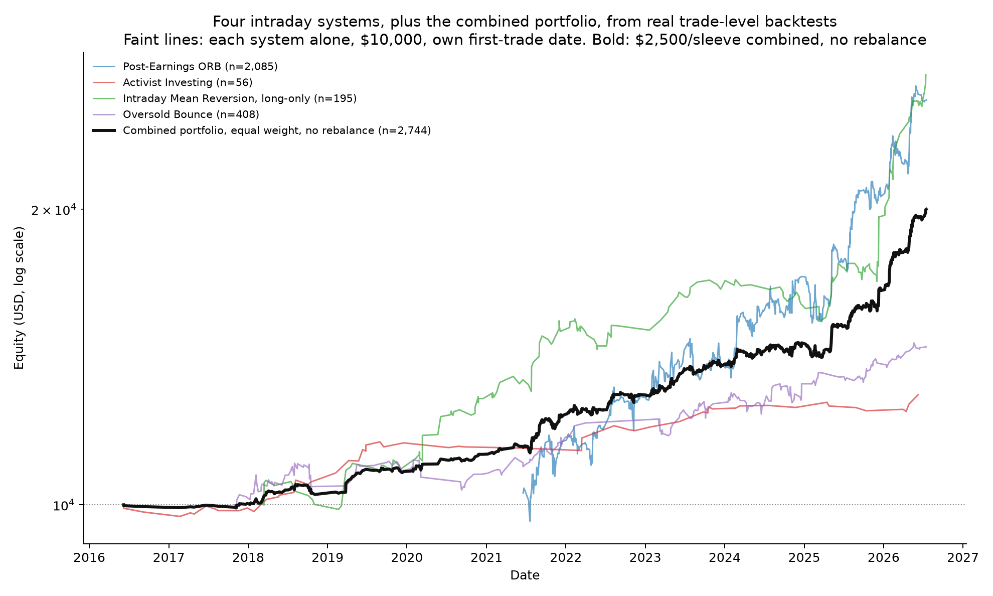
Faint lines: each system alone, $10,000, own first-trade date, verified track record in its section below. Log scale. Intraday Mean Reversion is the long-only book (a long+short combined variant was tested but its trade-level output could not be located for this entry, see that section). Bold black: the combined portfolio, described next.
The combined portfolio. $10,000 split into four $2,500 sleeves, one per system, each sleeve idle until its own system’s first real trade, then compounding on that system’s own real daily returns, no rebalancing between sleeves and no netting across systems. Real trade-level data end to end, summed on a unified date grid rather than estimated: $10,000 → $20,002 over 2016-06-07 to 2026-07-16 (10.1 years) · CAGR +7.1% · Sharpe 1.71 · Sortino 3.40 · Calmar 2.09 · max drawdown −3.4%. That drawdown is the headline number: every individual system’s own max drawdown (−10.3%, −2.1%, −9.3%, −6.8%) is worse than the combined portfolio’s, and the combined Sharpe is higher than any single system’s. Four systems with different triggers, different holding logic and different failure modes rarely draw down at the same time; that’s the entire case for running more than one of them.
1. Post-Earnings ORB (30-min Opening Range Breakout)
Hypothesis. An earnings gap generates continuation, not reversion. The opening range (9:30–10:00) is the auction trying to contain the imbalance; a break of that range confirms the imbalance is still live. The final system trades the break with a liquidity filter, an exhaustion filter, and a volatility-targeted sizing model; the exact thresholds aren’t published here.
What was tested and died (18 hypotheses). The market-cap gradient held again: edge lives in micro and small caps and drops to zero in mega caps, the sixth time this project has run into that exact pattern. Pre-market volume and RVOL as filters showed no stable structure. The entire short side, roughly 30 parameter cells, produced nothing; the short is not the mirror of the long here. Eleven variants of active trade management all lost to simply holding to the close. A tighter opening range with tighter stops won in-sample and reversed out-of-sample. Stacking the catalyst-scoring skill on top of the system was an untested interaction that came back at AUC 0.52, noise; the ORB does not need it.
The bug. Earnings-timing classification (before-open vs. after-close) came from Benzinga timestamps, which misclassified 23% of events as “intra-session,” which is not a real category. Rebuilding the session date from the acceptance timestamp on the company’s own SEC EDGAR 8-K filing, across roughly 200,000 filings, dropped the trades that had no real 8-K behind them, about a quarter of the original set, and the result improved once they were gone.
Final result, verified against the trade-level file. The source workbook’s own period, once corrected for the EDGAR filing dates, is 2021-06-18 to 2026-07-16 (about 5.1 calendar years, not the wider 2018–2026 window we started this write-up assuming), and it holds 2,085 trades, not the 1,653 originally cited.
$10,000 → $25,837 · total return +158.4% · CAGR +19.9% (computed from the verified daily curve) · Sharpe 1.22 · Sortino 2.06 · Calmar 1.93 · max drawdown −10.3% · 2,085 trades. Win rate 51.9%, but only 12.3% of trades actually hit the stop; the rest close somewhere between entry and stop at 4pm. The workbook’s own notes flag two things worth carrying forward: the 2021–2023 window is where the system was optimized, so the only clean read is the held-out 2024–2026 slice, +0.048R average (t = +2.38); and roughly 2,548 tickers in the original dataset never filed an 8-K in EDGAR (likely foreign private issuers filing a 6-K instead) and were dropped from the universe without checking whether that drop biases the result.
Why it works, if it works. The opening range is the market’s own attempt to absorb the earnings surprise in the first thirty minutes. A break of that range, on real volume, says the absorption failed and the imbalance is still being priced.
2. Activist Investing — Breaking News
Hypothesis. Headlines reporting an activist building a stake (accumulation language, sales explicitly excluded) generate an intraday upward drift that’s tradeable on the break of the first bar after the headline prints.
What was tested and died. The raw version, entering at the high of the two-minute bar after the headline and holding to the close, returned −48.2% net of realistic friction over the sample. No edge. Five pure-momentum exit variants (fixed target-to-stop ratios, EMA trailing stops) collapsed the same way: the entry-to-stop range was so small, a median of $0.10 per share, that two cents of round-trip slippage consumed roughly a fifth of the risk on half the trades. That’s scalping inside the bid-ask noise of the print, not trading a signal.
The turning point. One case flagged during review showed the headline did carry real edge, but the two-cent stop lived inside the noise of the move itself, and it stopped the trade out at −1R a moment before the stock ran five times that in the intended direction. Filtering by the reaction volume of the bar right after the headline against its own baseline, and widening the stop to a multiple of that same bar’s range, produced an edge that scaled monotonically with volume conviction.
A bug we caught ourselves. The first version of that volume filter summed volume from bars after entry, look-ahead bias. Corrected to use only the volume of the first bar that closes after the headline, the edge survived intact; it hadn’t been inflated by the leak.
A negative robustness test. Loosening the keyword filter to capture more trades per year (generic activist language, M&A chatter, FDA mentions) destroys the edge entirely. Whatever this is, it’s specific to the activist-campaign catalyst with genuine continuation behind it, not a generic “volume spike after a headline” effect.
Final result, causal system, no look-ahead, verified against the trade-level file. A liquidity-filtered, volume-conviction breakout with a fixed multiple-R target and fixed risk per trade; the exact thresholds aren’t published here. The file’s own dates run 2016-06-07 to 2026-06-09, about 10.0 years (not quite the ~10.5 originally cited), 56 trades, about 5.6 per year.
n = 56 · win rate 51.8% · expectancy +0.469R/trade · profit factor 2.82 (verified directly; the figure we started from, 2.59, did not match the file and is superseded by this one) · $10,000 → $12,946, +29.5% net of friction · max drawdown −2.1% (also revised from the figure we started with, −2.7%). Removing the three largest winners by R-multiple (each near the fixed target), expectancy holds at +0.327R/trade, independently recomputed from the trade file and matching the +0.325R originally reported. Low frequency, about 5.6 trades a year: this reads as a precision instrument, not something meant to fire often.
Why it works, if it works. An activist stake-building headline is a real, observed change in who owns the float, not a forecast; the volume filter is there to separate genuine institutional reaction from a headline nobody traded.
3. Intraday Mean Reversion
Hypothesis. In an actively declining, high-volume name, when sellers accelerate and get sloppy, a single green candle breaking the highs of two or more prior bars without waiting for a close, there’s a buyable snapback. The sloppiness is what gives the edge, not the extension by itself.
What was tested and died. The unfiltered pattern showed edge at 0–5bps of assumed slippage and died at 10bps, living inside the spread, the same failure mode as the ORB’s original bug. Measuring the real NBBO half-spread per trade instead of a flat assumption, the raw pattern nets negative, −0.109R. The two factors the starting hypothesis already specified do survive: a stretched-band filter on the long side and a volume-conviction filter on the short side; combined, they hold at +0.239R, robustly.
A methodology finding that validates the entry rule. Filtering by traits of the breakout candle itself, how far it had already closed, how large it was, looked spectacular in isolation, +0.48R. But those are outcome variables: they measure how far the candle had already moved before you could have measured it. Simulating an honest entry at that candle’s close instead of on the break, the edge collapsed to +0.014R. That’s exactly what the starting rule says: enter on the break, don’t wait for the close. Waiting kills the edge; the backtest now shows why.
Long-side refinement. It isn’t the extension by itself, it’s the speed of the final leg down into the low. A simplified, single exit rule improves on the original scale-out plan. Filtering by catalyst confirms the underlying thesis: earnings-driven setups lose (−0.083R, prior post-earnings drift working against the trade), while pure technical setups with no dated catalyst outperform (+0.462R). The edge here lives in technical noise, not in fundamentals.
Short side. This contradicts an earlier project’s finding that the extension fade dies on borrow cost; here the short with candle confirmation survives, in both easy-to-borrow and hard-to-borrow names alike, but decays hard out of sample, strong only in 2018–2021 and during COVID, flat since 2022. We do not have a verified trade-level file for a combined long+short book at the time of writing; the previously cited combined figures ($34,706 final equity, Sharpe 1.56) could not be reconciled against source data for this entry and are held out pending that file.
Final result, long side only, verified against the trade-level file (the cleanest version, no borrow required). A liquidity-filtered, time-of-day-windowed version with catalyst days excluded; the exact thresholds aren’t published here. Period 2018-03-14 to 2026-07-14 (about 8.3 years):
$10,000 → $27,435 · CAGR +12.9% · Sharpe 1.41 (file-reported and independently reproduced from the daily trade series) · Sortino 3.80 (independently computed, not in the original file) · Calmar 1.39 · max drawdown −9.3% · 195 trades, about 23/year · win rate 61.0% · expectancy +0.535R/trade.
Why it works, if it works. A sloppy break of a decline’s structure, confirmed on the print rather than the close, catches short covering before the market has time to decide whether the selling pressure is actually exhausted.
4. Bounce Play — Oversold Bounce (exhaustion gap-down)
Hypothesis. Buying an intraday oversold condition, a technical gap-down in an already beaten-up name, carries extra tailwind from the equity risk premium, without the locate restriction that caps the short side’s capacity.
The premise didn’t hold, but the strategy survived for a different reason. Measured open-to-close, the intraday drift is slightly negative; the risk premium lives overnight, not intraday, so that part of the original hypothesis does not hold as designed. What did work: a deep, multi-day oversold decline combined with a capitulation-volume day, a pure-technical filter (no recent 8-K at all), and excluding mega caps, since institutional ownership stability makes a large name’s decline more credible, not less, so large names tend to continue rather than bounce.
The hardest finding of the study. The first backtest window (2023–2026) showed a 2.2 Sharpe and looked like a clean edge, but it contained no sustained crash. Extended back to include 2018–2026 in full, including COVID, the raw, uncapped strategy is negative overall and March 2020 alone is a real disaster inside it (roughly −0.14R average and a 32% win rate during that stretch): buying the dip every session through a sustained waterfall destroys the account. The fix that resolves most of this is a practical cap on positions per day, chosen by liquidity rather than predictive ranking (every ranking scheme tested lost to picking at random), because it keeps the system out of the illiquid names that are the ones that don’t actually bounce. An optional regime filter, trading only in a favorable broad-market trend, improves drawdown, not Sharpe.
A caveat that remains open. Delisted-stock coverage in the data is thin, roughly 0.3% of the universe, which likely inflates the measured edge; the “falling knives” that ended in delisting are underrepresented in what we can test.
Final result, verified against the trade-level file. The verified source file uses a specific risk-per-trade and position-count configuration that differs from an earlier, lower-risk variant referenced earlier in this project; that specific file was not available at the time of writing, and the numbers below are the ones that could be verified, not the earlier estimate. Period 2017-11-01 to 2026-07-15 (about 8.7 years, spanning the full COVID window):
$10,000 → $14,485 · CAGR +4.35% · Sharpe 0.78 (independently computed from the daily curve; not in the source file) · Sortino 1.21 (same) · Calmar 0.64 · max drawdown −6.8% · 408 trades · win rate 58.6% · average +0.052R/trade. The position cap and liquidity filter hold up through the full COVID window in this configuration; whether the regime filter is doing meaningful additional work here, versus the position cap alone, is not separated out in this file.
Why it works, if it works. It’s a liquidity story more than a risk-premium story: capping exposure to a small number of liquid, real setups a day removes the illiquid, low-quality gap-downs that don’t actually mean-revert, which is most of what makes the raw, uncapped version dangerous.
What the four processes have in common
None of these four systems started as the version that survives above. Every one of them went through a version that looked good and wasn’t, for a reason specific to that system: a timestamp that didn’t match the true trigger, a look-ahead leak in a volume filter, an outcome variable disguised as a predictor, a sample window that happened to skip the one regime that would have broken it. The common thread isn’t a single number or rule; it’s three habits that kept showing up regardless of which system was being tested.
Every timestamp used as an order variable has to be checked against the entry timestamp specifically, not just checked for existing. A filing date, a headline print time, a volume bar’s close, each one has to be provably knowable before the trade it’s supposed to inform, not just recorded somewhere in the same dataset.
A result has to survive out of sample and across both halves of the test period before it counts as a result. In-sample wins that reverse out of sample showed up in two of these four systems (the ORB’s tighter opening range, the mean-reversion system’s close-entry variant); a short sample window hid the one regime, COVID, that would have broken the Bounce system’s raw version.
And the default posture toward a good-looking number is that it’s wrong until proven otherwise, including the numbers in this entry. Two of the four systems’ headline results changed between the first draft of this write-up and the version above, once we went back to the actual trade-level files instead of trusting the summary we started with. That’s not a footnote to the process described above; it’s the same process, applied one more time, to this document.
Pasamos las últimas semanas desarmando cuatro hipótesis intradía: una ruptura de rango de apertura tras earnings, un momentum por titulares de activistas 13D, un scalp de rebote por reversión a la media intradía, y una reversión a la media por sobreventa. Esta entrada documenta el proceso, no solo a los sobrevivientes. Matar una hipótesis que no se sostiene fuera de muestra es el trabajo real; los sistemas que lo lograron son lo que queda después de ese trabajo, no el punto del mismo. Donde una prueba no mostró edge, o donde nuestra propia metodología tuvo un bug, eso recibe la misma cantidad de palabras que las victorias.
Una nota sobre los propios límites de esta entrada, en el espíritu de la pieza: las cifras de resumen de las que partimos no todas cuadraron limpiamente contra los archivos de backtest a nivel de operación cuando volvimos a revisarlas. Donde divergieron, las cifras de abajo son las verificadas directamente contra los workbooks fuente, no las recordadas originalmente. Dos de los cuatro sistemas cambiaron como resultado, y eso se revela en línea, sistema por sistema, en vez de suavizarse. Y una nota aparte sobre el alcance: los umbrales exactos de entrada y salida detrás de cada sistema se retienen aquí a propósito; son la parte operable del edge, no el hallazgo de investigación, y son el tipo de detalle que preferimos poner detrás de una futura suscripción antes que regalarlo en un artículo público.
Líneas tenues: cada sistema solo, $10,000, su propia fecha de primera operación, track record verificado en su sección más abajo. Escala logarítmica. Intraday Mean Reversion es el libro solo-long (se probó una variante combinada long+short pero su salida a nivel de operación no pudo localizarse para esta entrada, ver esa sección). Negro en negrita: el portafolio combinado, descrito a continuación.
El portafolio combinado. $10,000 repartidos en cuatro sleeves de $2,500, uno por sistema, cada sleeve inactivo hasta la primera operación real de su propio sistema, luego componiendo sobre los retornos diarios reales de ese sistema, sin rebalanceo entre sleeves y sin neteo entre sistemas. Datos reales a nivel de operación de principio a fin, sumados sobre una malla de fechas unificada en vez de estimados: $10,000 → $20,002 durante 2016-06-07 a 2026-07-16 (10.1 años) · CAGR +7.1% · Sharpe 1.71 · Sortino 3.40 · Calmar 2.09 · drawdown máximo −3.4%. Ese drawdown es la cifra destacada: el drawdown máximo de cada sistema individual (−10.3%, −2.1%, −9.3%, −6.8%) es peor que el del portafolio combinado, y el Sharpe combinado es más alto que el de cualquier sistema solo. Cuatro sistemas con disparadores distintos, lógicas de holding distintas y modos de falla distintos rara vez caen al mismo tiempo; ese es todo el argumento para correr más de uno.
1. Post-Earnings ORB (ruptura de rango de apertura de 30 min)
Hipótesis. Un gap de earnings genera continuación, no reversión. El rango de apertura (9:30–10:00) es la subasta tratando de contener el desequilibrio; una ruptura de ese rango confirma que el desequilibrio sigue vivo. El sistema final opera la ruptura con un filtro de liquidez, un filtro de agotamiento, y un modelo de tamaño ajustado por volatilidad; los umbrales exactos no se publican aquí.
Lo que se probó y murió (18 hipótesis). El gradiente de capitalización se mantuvo otra vez: el edge vive en micro y small caps y cae a cero en mega caps, la sexta vez que este proyecto se topa con ese patrón exacto. El volumen premercado y el RVOL como filtros no mostraron estructura estable. Todo el lado short, unas 30 celdas de parámetros, no produjo nada; el short no es el espejo del long aquí. Once variantes de gestión activa de la operación perdieron todas contra simplemente sostener hasta el cierre. Un rango de apertura más estrecho con stops más ajustados ganó dentro de muestra y se revirtió fuera de muestra. Apilar el skill de puntuación de catalizadores sobre el sistema fue una interacción no probada que volvió con AUC 0.52, ruido; el ORB no lo necesita.
El bug. La clasificación del timing de earnings (antes de apertura vs. después del cierre) venía de timestamps de Benzinga, que clasificaron mal el 23% de los eventos como “intra-sesión”, que no es una categoría real. Reconstruir la fecha de sesión desde el timestamp de aceptación del propio 8-K de la empresa en SEC EDGAR, a través de unos 200,000 filings, eliminó las operaciones que no tenían un 8-K real detrás, cerca de un cuarto del conjunto original, y el resultado mejoró una vez que se fueron.
Resultado final, verificado contra el archivo a nivel de operación. El propio período del workbook fuente, una vez corregido por las fechas de filing de EDGAR, es 2021-06-18 a 2026-07-16 (unos 5.1 años calendario, no la ventana más amplia 2018–2026 con la que empezamos asumiendo este artículo), y contiene 2,085 operaciones, no las 1,653 citadas originalmente.
$10,000 → $25,837 · retorno total +158.4% · CAGR +19.9% (calculado desde la curva diaria verificada) · Sharpe 1.22 · Sortino 2.06 · Calmar 1.93 · drawdown máximo −10.3% · 2,085 operaciones. Tasa de acierto 51.9%, pero solo el 12.3% de las operaciones realmente tocó el stop; el resto cierra en algún punto entre la entrada y el stop a las 4pm. Las propias notas del workbook señalan dos cosas que vale la pena llevar adelante: la ventana 2021–2023 es donde se optimizó el sistema, así que la única lectura limpia es el tramo held-out 2024–2026, +0.048R promedio (t = +2.38); y unos 2,548 tickers del conjunto original nunca presentaron un 8-K en EDGAR (probablemente emisores privados extranjeros que presentan un 6-K en su lugar) y fueron eliminados del universo sin verificar si eso sesga el resultado.
Por qué funciona, si funciona. El rango de apertura es el propio intento del mercado de absorber la sorpresa de earnings en los primeros treinta minutos. Una ruptura de ese rango, con volumen real, dice que la absorción falló y el desequilibrio se sigue precificando.
2. Activist Investing, titulares de última hora
Hipótesis. Titulares que reportan que un activista está construyendo una posición (lenguaje de acumulación, ventas explícitamente excluidas) generan un drift intradía al alza que es operable en la ruptura de la primera vela después de que se publica el titular.
Lo que se probó y murió. La versión cruda, entrando en el máximo de la vela de dos minutos después del titular y sosteniendo hasta el cierre, devolvió −48.2% neto de fricción realista sobre la muestra. Sin edge. Cinco variantes de salida de puro momentum (ratios fijos de objetivo a stop, stops de trailing con EMA) colapsaron de la misma forma: el rango de entrada a stop era tan pequeño, una mediana de $0.10 por acción, que dos centavos de slippage de ida y vuelta consumían aproximadamente un quinto del riesgo en la mitad de las operaciones. Eso es hacer scalping dentro del ruido de bid-ask del titular, no operar una señal.
El punto de inflexión. Un caso señalado durante la revisión mostró que el titular sí llevaba edge real, pero el stop de dos centavos vivía dentro del ruido del propio movimiento, y sacó la operación en −1R un momento antes de que la acción corriera cinco veces eso en la dirección esperada. Filtrando por el volumen de reacción de la vela justo después del titular contra su propia línea base, y ampliando el stop a un múltiplo del rango de esa misma vela, se produjo un edge que escalaba monótonamente con la convicción de volumen.
Un bug que atrapamos nosotros mismos. La primera versión de ese filtro de volumen sumaba volumen de velas después de la entrada, sesgo de look-ahead. Corregido para usar solo el volumen de la primera vela que cierra después del titular, el edge sobrevivió intacto; no había sido inflado por la fuga.
Una prueba de robustez negativa. Ampliar el filtro de palabras clave para capturar más operaciones al año (lenguaje activista genérico, ruido de M&A, menciones de FDA) destruye el edge por completo. Sea lo que sea esto, es específico del catalizador de campaña activista con continuación genuina detrás, no un efecto genérico de “pico de volumen tras un titular”.
Resultado final, sistema causal, sin look-ahead, verificado contra el archivo a nivel de operación. Una ruptura filtrada por liquidez y convicción de volumen con un objetivo fijo de múltiplo de R y riesgo fijo por operación; los umbrales exactos no se publican aquí. Las propias fechas del archivo corren 2016-06-07 a 2026-06-09, unos 10.0 años (no exactamente los ~10.5 citados originalmente), 56 operaciones, unas 5.6 al año.
n = 56 · tasa de acierto 51.8% · expectativa +0.469R/operación · profit factor 2.82 (verificado directamente; la cifra de la que partimos, 2.59, no coincidía con el archivo y queda reemplazada por esta) · $10,000 → $12,946, +29.5% neto de fricción · drawdown máximo −2.1% (también revisado desde la cifra con la que partimos, −2.7%). Removiendo las tres mayores ganadoras por múltiplo de R (cada una cerca del objetivo fijo), la expectativa se sostiene en +0.327R/operación, recalculada de forma independiente desde el archivo de operaciones y coincidiendo con el +0.325R reportado originalmente. Baja frecuencia, unas 5.6 operaciones al año: esto se lee como un instrumento de precisión, no algo pensado para dispararse seguido.
Por qué funciona, si funciona. Un titular de construcción de posición activista es un cambio real y observado de quién es dueño del float, no un pronóstico; el filtro de volumen está ahí para separar la reacción institucional genuina de un titular que nadie operó.
3. Intraday Mean Reversion
Hipótesis. En un nombre en declive activo y de alto volumen, cuando los vendedores aceleran y se ponen descuidados, una sola vela verde que rompe los máximos de dos o más velas previas sin esperar un cierre, hay un rebote comprable. Lo descuidado es lo que da el edge, no la extensión por sí sola.
Lo que se probó y murió. El patrón sin filtrar mostró edge a 0–5bps de slippage asumido y murió a 10bps, viviendo dentro de la horquilla, el mismo modo de falla que el bug original del ORB. Midiendo la media horquilla NBBO real por operación en vez de un supuesto plano, el patrón crudo neto es negativo, −0.109R. Los dos factores que la hipótesis inicial ya especificaba sí sobreviven: un filtro de banda estirada en el lado long y un filtro de convicción de volumen en el lado short; combinados, se sostienen en +0.239R, de forma robusta.
Un hallazgo metodológico que valida la regla de entrada. Filtrar por rasgos de la propia vela de ruptura, qué tan lejos ya había cerrado, qué tan grande era, se veía espectacular en aislamiento, +0.48R. Pero esas son variables de resultado: miden qué tanto ya se había movido la vela antes de que se pudiera haber medido. Simulando una entrada honesta en el cierre de esa vela en vez de en la ruptura, el edge colapsó a +0.014R. Eso es exactamente lo que dice la regla inicial: entra en la ruptura, no esperes el cierre. Esperar mata el edge; el backtest ahora muestra por qué.
Refinamiento del lado long. No es la extensión por sí sola, es la velocidad de la última pierna de bajada hacia el mínimo. Una regla de salida simplificada y única mejora sobre el plan original de salida escalonada. Filtrar por catalizador confirma la tesis subyacente: los setups impulsados por earnings pierden (−0.083R, el drift post-earnings previo trabajando en contra de la operación), mientras que los setups puramente técnicos sin catalizador fechado superan (+0.462R). El edge aquí vive en el ruido técnico, no en los fundamentales.
Lado short. Esto contradice el hallazgo de un proyecto anterior de que el fade de extensión muere por costo de borrow; aquí el short con confirmación de vela sobrevive, tanto en nombres fáciles como difíciles de tomar prestado, pero decae fuerte fuera de muestra, fuerte solo en 2018–2021 y durante COVID, plano desde 2022. No tenemos un archivo verificado a nivel de operación para un libro combinado long+short al momento de escribir esto; las cifras combinadas citadas previamente ($34,706 de equity final, Sharpe 1.56) no pudieron reconciliarse contra datos fuente para esta entrada y quedan pendientes de ese archivo.
Resultado final, solo lado long, verificado contra el archivo a nivel de operación (la versión más limpia, sin necesidad de borrow). Una versión filtrada por liquidez y acotada por ventana horaria con días de catalizador excluidos; los umbrales exactos no se publican aquí. Período 2018-03-14 a 2026-07-14 (unos 8.3 años):
$10,000 → $27,435 · CAGR +12.9% · Sharpe 1.41 (reportado por el archivo y reproducido de forma independiente desde la serie diaria de operaciones) · Sortino 3.80 (calculado de forma independiente, no está en el archivo original) · Calmar 1.39 · drawdown máximo −9.3% · 195 operaciones, unas 23/año · tasa de acierto 61.0% · expectativa +0.535R/operación.
Por qué funciona, si funciona. Una ruptura descuidada de la estructura de un declive, confirmada en el print en vez de en el cierre, atrapa el cubrimiento de cortos antes de que el mercado tenga tiempo de decidir si la presión vendedora realmente se agotó.
4. Bounce Play, rebote por sobreventa (gap-down de agotamiento)
Hipótesis. Comprar una condición de sobreventa intradía, un gap-down técnico en un nombre ya golpeado, lleva un viento de cola extra de la prima de riesgo de renta variable, sin la restricción de localización que limita la capacidad del lado short.
La premisa no se sostuvo, pero la estrategia sobrevivió por otra razón. Medido de apertura a cierre, el drift intradía es levemente negativo; la prima de riesgo vive overnight, no intradía, así que esa parte de la hipótesis original no se sostiene tal como se diseñó. Lo que sí funcionó: un declive de sobreventa profundo y de varios días combinado con un día de volumen de capitulación, un filtro puramente técnico (sin 8-K reciente en absoluto), y excluir mega caps, ya que la estabilidad de la propiedad institucional hace que el declive de un nombre grande sea más creíble, no menos, así que los nombres grandes tienden a continuar en vez de rebotar.
El hallazgo más difícil del estudio. La primera ventana de backtest (2023–2026) mostró un Sharpe de 2.2 y se veía como un edge limpio, pero no contenía ningún crash sostenido. Extendida hacia atrás para incluir 2018–2026 completo, incluido COVID, la estrategia cruda y sin tope es negativa en general y marzo de 2020 por sí solo es un desastre real adentro (aproximadamente −0.14R promedio y una tasa de acierto de 32% durante ese tramo): comprar la caída cada sesión durante una cascada sostenida destruye la cuenta. El arreglo que resuelve la mayor parte de esto es un tope práctico de posiciones por día, elegido por liquidez en vez de ranking predictivo (todo esquema de ranking probado perdió contra elegir al azar), porque mantiene al sistema fuera de los nombres ilíquidos que son los que realmente no rebotan. Un filtro de régimen opcional, operando solo en una tendencia de mercado amplio favorable, mejora el drawdown, no el Sharpe.
Una salvedad que sigue abierta. La cobertura de acciones deslistadas en los datos es delgada, cerca del 0.3% del universo, lo cual probablemente infla el edge medido; los “cuchillos cayendo” que terminaron en deslistado están subrepresentados en lo que se puede probar.
Resultado final, verificado contra el archivo a nivel de operación. El archivo fuente verificado usa una configuración específica de riesgo por operación y conteo de posiciones que difiere de una variante anterior de menor riesgo referida antes en este proyecto; ese archivo específico no estaba disponible al momento de escribir esto, y las cifras de abajo son las que pudieron verificarse, no la estimación anterior. Período 2017-11-01 a 2026-07-15 (unos 8.7 años, abarcando la ventana completa de COVID):
$10,000 → $14,485 · CAGR +4.35% · Sharpe 0.78 (calculado de forma independiente desde la curva diaria; no está en el archivo fuente) · Sortino 1.21 (lo mismo) · Calmar 0.64 · drawdown máximo −6.8% · 408 operaciones · tasa de acierto 58.6% · promedio +0.052R/operación. El tope de posiciones y el filtro de liquidez se sostienen a través de la ventana completa de COVID en esta configuración; si el filtro de régimen está haciendo trabajo adicional significativo aquí, versus el tope de posiciones solo, no está separado en este archivo.
Por qué funciona, si funciona. Es más una historia de liquidez que una historia de prima de riesgo: acotar la exposición a un pequeño número de setups reales y líquidos por día remueve los gap-downs ilíquidos y de baja calidad que en realidad no revierten a la media, que es la mayor parte de lo que hace peligrosa a la versión cruda y sin tope.
Lo que los cuatro procesos tienen en común
Ninguno de estos cuatro sistemas empezó como la versión que sobrevive arriba. Cada uno de ellos pasó por una versión que se veía bien y no lo era, por una razón específica de ese sistema: un timestamp que no coincidía con el disparador verdadero, una fuga de look-ahead en un filtro de volumen, una variable de resultado disfrazada de predictor, una ventana de muestra que resultó saltarse el único régimen que la habría roto. El hilo común no es un número o una regla única; son tres hábitos que siguieron apareciendo sin importar qué sistema se estuviera probando.
Cada timestamp usado como variable de orden tiene que verificarse contra el timestamp de entrada específicamente, no solo verificarse que exista. Una fecha de filing, la hora de impresión de un titular, el cierre de una vela de volumen, cada uno tiene que ser demostrablemente conocible antes de la operación que se supone que debe informar, no solo estar registrado en algún lugar del mismo dataset.
Un resultado tiene que sobrevivir fuera de muestra y a través de ambas mitades del período de prueba antes de que cuente como un resultado. Las victorias dentro de muestra que se revierten fuera de muestra aparecieron en dos de estos cuatro sistemas (el rango de apertura más estrecho del ORB, la variante de entrada al cierre del sistema de reversión a la media); una ventana de muestra corta escondió el único régimen, COVID, que habría roto la versión cruda del sistema Bounce.
Y la postura por defecto ante un número que se ve bien es que está mal hasta que se demuestre lo contrario, incluidos los números de esta entrada. Los resultados destacados de dos de los cuatro sistemas cambiaron entre el primer borrador de este artículo y la versión de arriba, una vez que volvimos a los archivos reales a nivel de operación en vez de confiar en el resumen con el que partimos. Eso no es una nota al pie del proceso descrito arriba; es el mismo proceso, aplicado una vez más, a este documento.